Initialization Of Deep Networks Case of Rectifiers

Introduction

Recent success in deep networks can be credited to the use of non-saturated activation function Rectified Linear unit (RReLu) which has replaced its saturated counterpart (e.g. sigmoid, tanh). Benefits associated with the ReLu activation function include:

• Ability to mitigate the exploding or vanishing gradient problem; this largely due to the fact that for all inputs into the activation function of values grater than $0$, the gradient is always $1$ (constant gradient)
• The constant gradient of ReLu activations results in faster learning. This helps expedite convergence of the training procedure yielding better better solutions than sigmoidlike units
• Unlike the sigmoidlike units (such as sigmoid or tanh activations) ReLu activations does not involve computing of an an exponent which is a factor that results to a faster training and evaluation times.
• Producing sparse representations with true zeros. All inputs into the activation function of values less than or equal to $0$, results in an output value of $0$. Sparse representations are considered more valuable

Xavier and Bengio (2010) [2] had earlier on proposed the “Xavier” initialization, a method whose derivation was based on the assumption that the activations are linear. This assumption however is invalid for ReLu and PReLu. He, Kaiming, et al. 2015 [1] later on derived a robust initialization method that particularly considers the rectifier nonlinearities.

In this article we discuss the algorithm put forward by He, Kaiming, et al. 2015 [1].

Notation

1. $k$ is the side length of a convolutional kernel. (also the spatial filter size of the layer)
2. $c$ is the channel number. (also input channel)
3. $n$ is the number of connections of a response ($n = k \times k \times c \implies k^2c$)
4. $\mathbf{x}$ is the co-located $k \times k$ pixels in $c$ inputs channels. ($\mathbf{x} = (k^2c) \times 1$)
5. $W$ is the matrix where $d$ is the total number number of filters. Every row of $W$ i.e $(d_1,d_2,\dotsb,d_d)$ represents the weights of a filter. ($W = d \times n$)
6. $\mathbf{b}$ is the vector of biases.
7. $\mathbf{y}$ is the response pixel of the output map
8. $l$ is used to index the layers
9. $f(\cdot)$ is the activation function
10. $\mathbf{x} = f(\mathbf{y}_{l-1}) \$
11. $c = d_{l-1} \$
12. $\mathbf{y}_l = W_l\mathbf{x}_l+\mathbf{b}_l \$

Forward Propagation Case

Considerations made here include:

• The initialized elements in $W_l$ be mutually independent and share the same distribution.
• The elements in $\mathbf{x}_l$ are mutually independent and share the same distribution.
• $\mathbf{x}_l$ and $W_l$ are independent of each other.

The variance of $y_l$ can be given by: $$ \begin{align} Var[y_l] &= n_lVar[w_lx_l], \tag 1 \end{align} $$

where $y_l, w_l, x_l$ represent random variables of each element in $\mathbf{y}_l, W_l, \mathbf{x}_l$. Let $w_l$ have a zero mean, then the variance of the product of independent variables gives us: $$ \begin{align} Var[y_l] &= n_lVar[w_l]E[x^2_l]. \tag 2 \end{align} $$

Lets look at how the Eqn. $(2)$ above is arrived at:-

For random variables $\mathbf{x}_l$ and $W_l$, independent of each other, we can use basic properties of expectation to show that: $$ \begin{align} Var[w_lx_l] &= E[w^2_l]E[x^2_l] - \overbrace{ \left[ E[x_l]\right]^2 \left[ E[w_l]\right]^2 }^{ \bigstar } , \tag {A} \end{align} $$

From Eqn. $(2)$ above, we let $w_l$ have a zero mean $\implies E[w_l] = \left[E[w_l]\right]^2 = 0$. This means that in Eqn. $(A)$, $\bigstar$ evaluates to zero. We are then left with: $$ \begin{align} Var[w_lx_l] &= E[w^2_l]E[x^2_l], \tag {B} \end{align} $$

Using the formula for variance $Var[w_l] = E[w^2_l] -\left[E[w_l]\right]^2$ and the fact that $E[w_l] = 0$ we come to the conclusion that $Var[w_l] = E[w^2_l]$.

With this conclusion we can replace $E[w^2_l]$ in Eqn. $(B)$ with $Var[w_l]$ to obtain the following Eqn.: $$ \begin{align} Var[w_lx_l] &= Var[w_l]E[x^2_l], \tag {C} \end{align} $$

By substituting Eqn. $(C)$ into Eqn. $(1)$ we obtain: $$ \begin{align} Var[y_l] &= n_lVar[w_l]E[x^2_l]. \tag 2 \end{align} $$

In Eqn. $(2)$ it is well worth noting that $E[x^2_l]$ is the expectation of the square of $x_l$ and cannot resolve to $Var[x_l]$ i.e $E[x^2_l] \neq Var[x_l]$ as we did above for $w_l$ unless $x_l$ has zero mean.

The effect of ReLu activation is such that $x_l = max(0, y_{l-1})$ and thus it does not have zero mean. For this reason the conclusion here is different compared to the initialization style in [2].

We can also observe here that despite the mean of $x_l$ i.e $E[x_l]$ being non zero, the product of the two means $E[x_l]$ and $E[w_l]$ will lead to a zero mean since $E[w_l] = 0$ as shown in the Eqn. below: $$ \begin{align} E[y_l] &= E[w_lx_l] = E[x_l]E[w_l] = 0. \end{align} $$

If we let $w_{l-1}$ have a symmetric distribution around zero and $b_{l-1} = 0$, then from our observation above $y_{l-1}$ has zero mean and a symmetric distribution around zero. This leads to $E[x^2_l] = \frac{1}{2}Var[y_{l-1}]$ when $f(\cdot)$ is ReLu. Putting this in Eqn. $(2)$, we obtain: $$ \begin{align} Var[y_l] &= n_lVar[w_l]\frac{1}{2}Var[y_{l-1}]. \tag 3 \end{align} $$

With $L$ layers put together, we have: $$ \begin{align} Var[y_L] &= Var[y_1]\left( \prod_{l=1}^L \frac{1}{2}n_lVar[w_l] \right). \tag 4 \end{align} $$

The product in Eqn. $\mathbf{(4)}$ is key to the initialization design.

Lets take some time to explain the effect of ReLu activation as seen in Eqn. $(3)$.

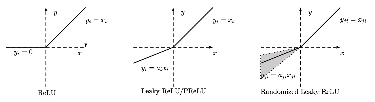
For the family of rectified linear (ReL) shown illustrated in the diagram above, we have a generic activation function defined as follows:

In the activation function $(5)$ above, $y_i$ is the input of the nonlinear activation $f$ on the $i$th channel, and $a_i$ is the coefficient controlling the slope of the negative part. $i$ in $a_i$ indicates that we allow the nonlinear activation to vary on different channels.

The variations of rectified linear (ReL) take the following forms:

1. ReLu: obtained when $a_i = 0$. The resultant activation function is of the form $f(y_i) = max(0,y_i)$
2. PReLu: Parametric ReLu - obtained when $a_i$ is a learnable parameter. The resultant activation function is of the form $f(y_i) = max(0,y_i) + a_i min(0,y_i)$
3. LReLu: Leaky ReLu - obtained when $a_i = 0.01$ i.e when $a_i$ is a small and fixed value [3]. The resultant activation function is of the form $f(y_i) = max(0,y_i) + 0.01 min(0,y_i)$
4. RReLu: Randomized Leaky ReLu - the randomized version of leaky ReLu, obtained when $a_{ji}$ is a random number sampled from a uniform distribution $U(l,u)$ i.e $a_{ji} \sim U(l, u); \, l < u \, \text{and} \, l, u \in [0; 1)$. See [2].

Rectifier activation function is simply a threshold at zero hence allowing the network to easily obtain sparse representations. For example, after uniform initialization of the weights, around $50\%$ of hidden units continuous output values are real zeros, and this fraction can easily increase with sparsity-inducing regularization [5].

Take signal $y_i = W_ix+b,$ (visualize the signal represented on a bi-dimensional space $y_i \in \mathbb{R}^2$). Applying the rectifier activation function to this signal i.e $f(y_i)$ where $f$ is ReLu results in a scenario where signals existing in regions where $y_i \lt 0$ are squashed to $0$, while those existing in regions where $y_i \gt 0$ remain unchanged.

The ReLu effect results in “aggressive data compression” where information is lost (replaced by real zeros values). A remedy for this would be the PReLu and LReLu implementations which provides an axle shift that adds a slope $a_i$ to the negative section ensuring from the data some information is retained rather than reduced to zero. Both PReLu and LReLu represented by variations of $f(y_i) = max(0,y_i) + a_i min(0,y_i)$, make use of the factor $a_i$ which serves as the component used to retain some information.

Using ReLu activation function function therefore, only the positive half axis values are obtained hence:

$\begin{align} E[x^2_l] &= \frac{1}{2}Var[y_{l-1}] \tag 6 \end{align} \ $

Putting this in Eqn. $(2)$, we obtain our Eqn. $(3)$ as above:

Note that a proper initialization method should avoid reducing and magnifying the magnitudes of input signals exponentially. For this reason we expect the product in Eqn. $(4)$ to take a proper scalar (e.g., 1). This leads to: $$ \begin{align} \frac{1}{2}n_lVar[w_l] &= 1, \quad \forall l \tag 7 \end{align} $$

From Eqn. $(7)$ above, we can conclude that: $$ \begin{align} Var[w_l] = \frac{2}{n_l} \implies \text{standard deviation (std)} = \sqrt{\frac{2}{n_l}} \end{align} $$

The initialization according to [1] is a zero-mean Gaussian distribution whose standard deviation (std) is $\sqrt{2/n_l}$. The bias is initialized to zero. The initialization distribution therefore is of the form: $$ \begin{align} W_l \sim \mathcal N \left({\Large 0}, \sqrt{\frac{2}{n_l}} \right) \,\text{and} \,\mathbf{b} = 0. \end{align} $$

From Eqn. $(4)$, we can observe that for the first layer $(l = 1)$, the variance of weights is given by $n_lVar[w_l] = 1$ because there is no ReLu applied on the input signal. However, the factor of a single layer does not make the overall product exponentially large or small and as such we adopt Eqn. $(7)$ in the first layer for simplicity.

Backward Propagation Case

For back-propagation, the gradient of the conv-layer is computed by: $$ \begin{align} \Delta{\mathbf{x}_l} &= W_l\Delta{\mathbf{y}_l}. \tag{8} \end{align} $$

Notation

1. $\Delta{\mathbf{x}_l}$ is the gradient $\frac{\partial \epsilon}{\partial \mathbf{x}}$
2. $\Delta{\mathbf{y}_l}$ is the gradient $\frac{\partial \epsilon}{\partial \mathbf{y}}$
3. $\Delta{\mathbf{y}_l}$ is represented by $k$ by $k$ pixels in $d$ channels and is thus reshaped into $k^2d$ by $1$ vector i.e $\Delta{\mathbf{y}_l} = k^2d \times 1$.
4. $\hat{n}$ is given by $k^2d$ also note that $\hat{n} \neq n$.
5. $\hat{W}$ is a $c \text{-by-} n$ matrix where filters are arranged in the back-propagation way. Also $\hat{W}$ and $W$ can be reshaped from each other.
6. $\Delta{\mathbf{x}}$ is a $c \text{-by-} 1$ vector representing the gradient at a pixel of this layer.

Assumptions made here include:

• Assume that $w_l$ and $\Delta{y_l}$ are independent of each other then $\Delta{x_l}$ has zero mean for all $l$, when $w_l$ is initialized by a symmetric distribution around zero.
• Assume that $f'(y_l)$ and $\Delta{x_{l+1}}$ are independent of each other

In back-propagation we have $\Delta{\mathbf{y}_l} = f'(y_l)\Delta{x_{l+1}}$ where $f'$ is the derivative of $f$. For the ReLu case $f'(y_l)$ is either zero or one with their probabilities being equal i.e $\Pr{(0)} = \frac{1}{2}$ and $\Pr{(1)} = \frac{1}{2}$.

Lets build on from some definition here; for a discrete case, the expected value of a discrete random variable, X, is found by multiplying each X-value by its probability and then summing over all values of the random variable. That is, if X is discrete, $$ \begin{align} E[X] &= \sum_{\text{all}\,x} xp(x) \end{align} $$

The expectation of $f'(y_l)$ then: $$ \begin{align} E[f’(y_l)] &= (0)\frac{1}{2} + (1)\frac{1}{2} = \frac{1}{2} \tag{9} \end{align} $$

With the independence of $f'(y_l)$ and $\Delta{x_{l+1}}$, we can show that: The expectation of $f'(y_l)$ then: $$ \begin{align} E[\Delta{y_{l}}] &= E[f’(y_l)\Delta{x_{l+1}}] = E[f’(y_l)]E[\Delta{x_{l+1}}] \tag{10} \end{align} $$

Substituting results in Eqn. $(9)$ into Eqn. $(10)$ we obtain: $$ \begin{align} E[\Delta{y_{l}}] &= \frac{1}{2}E[\Delta{x_{l+1}}] = 0 \tag{11} \end{align} $$

In Eqn. $(10)$ $\Delta{x_l}$ has zero mean for all $l$ which gives us the result zero. With this we can show that $E[(\Delta{y_{l}})^2] = Var[\Delta{y_{l}}]$ using the formula of variance as follows:

Again with the assumption that $\Delta{x_l}$ has zero mean for all $l$, we show can that the variance of product of two independent variables $f'(y_l)$ and $\Delta{x_{l+1}}$ to be

From the values of $f'(y_l) \in \lbrace 0,1 \rbrace$ we can observe that $1^2 = 1$ and $0^2 = 0$ meaning $f'(y_l) = [f'(y_l)]^2$.

This means that $E[f'(y_l)] = E[(f'(y_l))^2] = \frac{1}{2}$. Using this result in Eqn. $(12)$ we obtain:

Using the formula for variance and yet again the assumption that $\Delta{x_l}$ has zero mean for all $l$, we show can that $Var[\Delta{x_{l+1}}] = E[(\Delta{x_{l+1}})^2]$:

Substituting this result in Eqn. $(13)$ we obtain: $$ \begin{align} E[(\Delta{y_{l}})^2] &= Var[\Delta{y_{l}}] = \frac{1}{2}E[(\Delta{x_{l+1}})^2] \tag{15} \end{align} $$

The variance of Eqn. $(8)$ can be shown to be:

The scalar $1/2$ in both Eqn. $(16)$ and Eqn. $(3)$ is the result of ReLu, though the derivations are different. With $L$ layers put together, we have: $$ \begin{align} Var[\Delta{x_2}] &= Var[\Delta{x_{L+1}}]\left( \prod_{l=2}^L \frac{1}{2}\hat{n}_lVar[w_l] \right) \tag{17} \end{align} $$

Considering a sufficient condition that the gradient is not exponentially large/small: $$ \begin{align} \frac{1}{2}\hat{n}_lVar[w_l] &= 1, \quad \forall{l} \tag{18} \end{align} $$

The only difference between Eqn. $(18)$ and Eqn. $(7)$ is that $\hat{n} = k^2_ld_l$ while $n = k^2_lc_l = k^2_ld_{l-1}$. Eqn. $(18)$ results in a zero-mean Gaussian distribution whose standard deviation (std) is $\sqrt{2/\hat{n}_l}$. The initialization distribution therefore is of the form: $$ \begin{align} W_l \sim \mathcal N \left({\Large 0}, \sqrt{\frac{2}{\hat{n}_l}} \right) \end{align} $$

For the layer $(l = 1)$, we need not compute $\Delta{x}$ because it represents the image domain. We adopt Eqn. $(18)$ for the first layer for the same reason as the forward propagation case - the factor of a single layer does not make the overall product exponentially large or small.

It is noted that use of either Eqn. $(18)$ or Eqn. $(4)$ alone is sufficient. For example, if we use Eqn.$(18)$, then in Eqn. $(17)$ the product $\prod_{l=2}^L \frac{1}{2}\hat{n}_lVar[w_l] = 1$, and in Eqn. $(4)$ the product $\prod_{l=2}^L \frac{1}{2}n_lVar[w_l] = \prod_{l=2}^L n_l/\hat{n} = c_2/d_L$, which is not a diminishing number in common network designs. This means that if the initialization properly scales the backward signal, then this is also the case for the forward signal; and vice versa.

For initialization in the PReLu case, it is easy to show that Eqn. $(4)$ becomes: $$ \begin{align} \frac{1}{2}(1+a^2)n_lVar[w_l] &= 1, \tag {19} \end{align} $$

Where $a$ is the initialized value of the coefficients. If $a = 0$, it becomes the ReLu case; if $a = 1$, it becomes the linear case; same as [2]. Similarly, Eqn. $(14)$ becomes: $$ \begin{align} \frac{1}{2}(1+a^2)\hat{n}_lVar[w_l] &= 1, \tag {20} \end{align} $$

Applications

The initialization routines derived here, more famously known as “Kaiming Initialization” have been successfully applied in various deep learning libraries. Below we shall look at Keras a minimalist, highly modular neural networks library, written in Python and capable of running on top of either TensorFlow or Theano.

The initialization routine here is named “he_” following the name of one of the authors Kaiming He [1]. In the code snippet below, he_normal is the implementation of initialization based on Gaussian distribution while he_uniform is the equivalent implementation of initialization based on Uniform distribution

def get_fans(shape):
    fan_in = shape[0] if len(shape) == 2 else np.prod(shape[1:])
    fan_out = shape[1] if len(shape) == 2 else shape[0]
return fan_in, fan_out

def he_normal(shape, name=None):
    fan_in, fan_out = get_fans(shape)
    s = np.sqrt(2. / fan_in)
    return normal(shape, s, name=name)

def he_uniform(shape, name=None):
    fan_in, fan_out = get_fans(shape)
    s = np.sqrt(6. / fan_in)
return uniform(shape, s, name=name)

References

1. He, Kaiming, et al. “Delving deep into rectifiers: Surpassing human-level performance on imagenet classification.” Proceedings of the IEEE International Conference on Computer Vision. 2015. [PDF]
2. Glorot Xavier, and Yoshua Bengio. “Understanding the difficulty of training deep feedforward neural networks.” Aistats. Vol. 9. 2010. [PDF]
3. A. L. Maas, A. Y. Hannun, and A. Y. Ng. “Rectifier nonlinearities improve neural network acoustic models.” In ICML, 2013. [PDF]
4. Xu, Bing, et al. “Empirical Evaluation of Rectified Activations in Convolution Network.” [PDF]
5. Glorot, Xavier, Antoine Bordes, and Yoshua Bengio. “Deep Sparse Rectifier Neural Networks.” Aistats. Vol. 15. No. 106. 2011. [PDF]