Vanishing And Exploding Gradient Problems

Jefkine, 21 May 2018

Introduction

Two of the common problems associated with training of deep neural networks using gradient-based learning methods and backpropagation include the vanishing gradients and that of the exploding gradients.

In this article we explore how these problems affect the training of recurrent neural networks and also explore some of the methods that have been proposed as solutions.

Recurrent Neural Network

A recurrent neural network has the structure of multiple feedforward neural networks with connections among their hidden units. Each layer on the RNN represents a distinct time step and the weights are shared across time.

The combined feedfoward neural networks work over time to compute parts of the output one at a time sequentially.

Connections among the hidden units allow the model to iteratively build a relevant summary of past observations hence capturing dependencies between events that are several steps apart in the data.

An illustration of the RNN model is given below:

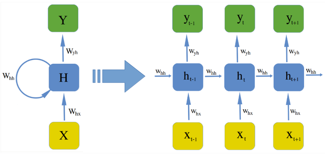
For any given time point $t$, the hidden state $\textbf{h}_{t}$ is computed using a function $f_{\textbf{W}}$ with parameters $\textbf{W}$ that takes in the current data point $\textbf{x}_{t}$ and hidden state in the previous time point $\textbf{h}_{t-1}$. i.e $f_{\textbf{W}}(\textbf{h}_{t-1}, \textbf{x}_{t})$.

$\textbf{W}$ represents a set of tunable parameters or weights on which the function $f_{\textbf{W}}$ depends. Note that the same weight matrix $\textbf{W}$ and function $f$ are used at every timestep.

Parameters $\textbf{W}$ control what will be remembered and what will be discarded about the past sequence allowing data points from the past say $\textbf{x}_{t - n}$ for $n \geq 1$ to influence the current and even later outputs by way of the recurrent connections

In its functional form, the recurrent neural network can be represented as:

$$\begin{align} \textbf{h}_{t} &= f_{\textbf{W}}\left(\textbf{h}_{t-1}, \textbf{x}_{t} \right) \tag{1} \\ \textbf{h}_{t} &= f\left(\textbf{W}_{hx}x_{t} + \textbf{W}_{hh}h_{t-1} + \textbf{b}_{h}\right) \tag{2a} \\ \textbf{h}_{t} &= \textbf{tanh}\left(\textbf{W}_{hx}x_{t} + \textbf{W}_{hh}h_{t-1} + \textbf{b}_{h}\right) \tag{2b} \\ \hat{\textbf{y}}_{t} &= \textbf{softmax}\left(\textbf{W}_{yh}h_{t} + \textbf{b}_{y}\right) \tag{3} \end{align}$$

From the above equations we can see that the RNN model is parameterized by three weight matrices

• $\textbf{W}_{hx} \in \mathbb{R}^{h \times x}$ is the weight matrix between input and the hidden layer
• $\textbf{W}_{hh} \in \mathbb{R}^{h \times h}$ is the weight matrix between two hidden layers
• $\textbf{W}_{yh} \in \mathbb{R}^{y \times h}$ is the weight matrix between the hidden layer and the output

We also have bias vectors incorporated into the model as well

• $\textbf{b}_{h} \in \mathbb{R}^{h}$ is the bias vector added to the hidden layer
• $\textbf{b}_{y} \in \mathbb{R}^{y}$ is the bias vector added to the output layer

$\textbf{tanh}(\cdot)$ is the non-linearity added to the hidden states while $\textbf{softmax}(\cdot)$ is the activation function used in the output layer.

RNNs are trained in a sequential supervised manner. For time step $t$, the error is given by the difference between the predicted and targeted: $(\hat{\textbf{y}_t} - \textbf{y}_{t})$. The overall loss $\mathcal{L}(\hat{\textbf{y}}, \textbf{y})$ is usually a sum of time step specific losses found in the range of intrest $[t, T]$ given by:

$$\begin{align} \mathcal{\large{L}} (\hat{\textbf{y}}, \textbf{y}) = \sum_{t = 1}^{T} \mathcal{ \large{L} }(\hat{\textbf{y}_t}, \textbf{y}_{t}) \tag{4} \end{align}$$

Vanishing and Exploding Gradients

Training of the unfolded recurrent neural network is done across multiple time steps using backpropagation where the overall error gradient is equal to the sum of the individual error gradients at each time step.

This algorithm is known as backpropagation through time (BPTT). If we take a total of $T$ time steps, the error is given by the following equation:

$$\begin{align} \frac{\partial \textbf{E}}{\partial \textbf{W}} = \sum_{t=1}^{T} \frac{\partial \textbf{E}_{t}}{\partial \textbf{W}} \tag{5} \end{align}$$

Applying chain rule to compute the overall error gradient we have the following

$$\begin{align} \frac{\partial \textbf{E}}{\partial \textbf{W}} = \sum_{t=1}^{T} \frac{\partial \textbf{E}}{\partial \textbf{y}_{t}} \frac{\partial \textbf{y}_{t}}{\partial \textbf{h}_{t}} \overbrace{\frac{\partial \textbf{h}_{t}}{\partial \textbf{h}_{k}}}^{ \bigstar } \frac{\partial \textbf{h}_{k}}{\partial \textbf{W}} \tag{6} \end{align}$$

The term marked $\bigstar$ ie $\frac{\partial \textbf{h}_{t}}{\partial \textbf{h}_{k}}$ is the derivative of the hidden state at time $t$ with respect to the hidden state at time $k$. This term involves products of Jacobians $\frac{\partial \textbf{h}_{i}}{\partial \textbf{h}_{i-1}}$ over subsequences linking an event at time $t$ and one at time $k$ given by:

$$\begin{align} \frac{\partial \textbf{h}_{t}}{\partial \textbf{h}_{k}} &= \frac{\partial \textbf{h}_{t}}{\partial \textbf{h}_{t-1}} \frac{\partial \textbf{h}_{t-1}}{\partial \textbf{h}_{t-2}} \cdots \frac{\partial \textbf{h}_{k+1}}{\partial \textbf{h}_{k}} \tag{7} \\ &= \prod_{i=k+1}^{t} \frac{\partial \textbf{h}_{i}}{\partial \textbf{h}_{i-1}} \tag{8} \end{align}$$

The product of Jacobians in Eq. $7$ features the derivative of the term $\textbf{h}_{t}$ w.r.t $\textbf{h}_{t-1}$, i.e $\frac{\partial \textbf{h}_{t}}{\partial \textbf{h}_{t-1}}$ which when evaluated on Eq. $2a$ yields $\textbf{W}^\top \left[ f'\left(\textbf{h}_{t-1}\right) \right]$, hence:

$$\begin{align} \prod_{i=k+1}^{t} \frac{\partial \textbf{h}_{i}}{\partial \textbf{h}_{i-1}} = \prod_{i=k+1}^{t} \textbf{W}^\top \text{diag} \left[ f'\left(\textbf{h}_{i-1}\right) \right] \tag{9} \end{align}$$

If we perform eigendecomposition on the Jacobian matrix $\frac{\partial \textbf{h}_{t}}{\partial \textbf{h}_{t-1}}$ given by $\textbf{W}^\top \text{diag} \left[ f'\left(\textbf{h}_{t-1}\right) \right]$, we get the eigenvalues $\lambda_{1}, \lambda_{2}, \cdots, \lambda_{n}$ where $\lvert\lambda_{1}\rvert \gt \lvert\lambda_{2}\rvert \gt\cdots \gt \lvert\lambda_{n}\rvert$ and the corresponding eigenvectors $\textbf{v}_{1},\textbf{v}_{1},\cdots,\textbf{v}_{n}$.

Any change on the hidden state $\Delta\textbf{h}_{t}$ in the direction of a vector $\textbf{v}_{i}$ has the effect of multiplying the change with the eigenvalue associated with this eigenvector i.e $\lambda_{i}\Delta\textbf{h}_{t}$.

The product of these Jacobians as seen in Eq. $9$ implies that subsequent time steps, will result in scaling the change with a factor equivalent to $\lambda_{i}^{t}$.

$\lambda_{i}^{t}$ represents the $\text{i}^{th}$ eigenvalue raised to the power of the current time step $t$.

Looking at the sequence $\lambda_{i}^{1}\Delta\textbf{h}_{1}, \lambda_{i}^{2}\Delta\textbf{h}_{2}, \cdots \lambda_{i}^{n}\Delta\textbf{h}_{n}$, it is easy to see that the factor $\lambda_{i}^{t}$ will end up dominating the $\Delta\textbf{h}_{t}$’s because this term grows exponentially fast as $\text{t} \rightarrow \infty$.

This means that if the largest eigenvalue $\lambda_{1} \lt 1$ then the gradient will vanish while if the value of $\lambda_{1} \gt 1$, the gradient explodes.

Alternate intuition: Lets take a deeper look at the norms associated with these Jacobians:

$$\begin{align} \left\lVert \frac{\partial \textbf{h}_{i}}{\partial \textbf{h}_{i-1}} \right\rVert \leq \left\lVert \textbf{W}^\top \right\rVert \left\lVert \text{diag} \left[ f'\left(\textbf{h}_{i-1}\right) \right] \right\rVert \tag{10} \end{align}$$

In Eq. $10$ above, we set $\gamma_{\textbf{W}}$, the largest eigenvalue associated with $\left\lVert \textbf{W}^\top \right\rVert$ as its upper bound, while $\gamma_{\textbf{h}}$ largest eigenvalue associated with $\left\lVert \text{diag} \left[ f'\left(\textbf{h}_{i-1}\right) \right] \right\rVert$ as its corresponding the upper bound.

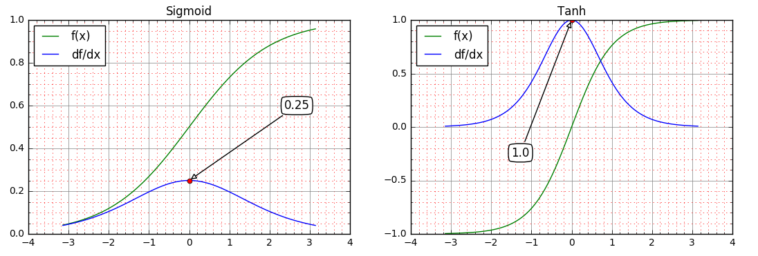
Depending on the activation function $f$ chosen for the model, the derivative $f'$ in $\left\lVert \text{diag} \left[ f'\left(\textbf{h}_{i-1}\right) \right] \right\rVert$ will be upper bounded by different values. For $\textbf{tanh}$ we have $\gamma_{\textbf{h}} = 1$ while for $\textbf{sigmoid}$ we have $\gamma_{\textbf{h}} = 1/4$. These two are illustrated in the diagrams below:

The chosen upper bounds $\gamma_{\textbf{W}}$ and $\gamma_{\textbf{h}}$ end up being a constant term resulting from their product as shown in Eq. $11$ below:

$$\begin{align} \left\lVert \frac{\partial \textbf{h}_{i}}{\partial \textbf{h}_{i-1}} \right\rVert \leq \left\lVert \textbf{W}^\top \right\rVert \left\lVert \text{diag} \left[ f'\left(\textbf{h}_{i-1}\right) \right] \right\rVert \leq \gamma_{\textbf{W}} \gamma_{\textbf{h}} \tag{11} \end{align}$$

The gradient $\frac{\partial \textbf{h}_{t}}{\partial \textbf{h}_{k}}$, as seen in Eq. $8$, is a product of Jacobian matrices that are multiplied many times, $t-k$ times to be precise in our case.

This relates well with Eq. $11$ above where the norm $\left\lVert \frac{\partial \textbf{h}_{t}}{\partial \textbf{h}_{k}} \right\rVert$ is essentially given by a constant term $\left( \gamma_{\textbf{W}} \gamma_{\textbf{h}} \right)$ to the power $t -k$ as shown below:

$$\begin{align} \left\lVert \frac{\partial \textbf{h}_{t}}{\partial \textbf{h}_{k}} \right\rVert = \left\lVert \prod_{i=k+1}^{t} \frac{\partial \textbf{h}_{i}}{\partial \textbf{h}_{i-1}} \right\rVert \leq \left( \gamma_{\textbf{W}} \gamma_{\textbf{h}} \right)^{t-k} \tag{12} \end{align}$$

As the sequence gets longer (i.e the distance between $t$ and $k$ increases), then the value of $\gamma$ will determine if the gradient either gets very large (explodes) on gets very small (vanishes).

Since $\gamma$ is associated with the leading eigenvalues of $\frac{\partial \textbf{h}_{i}}{\partial \textbf{h}_{i-1}}$, the recursive product of $t -k$ Jacobian matrices as seen in Eq. $12$ makes it possible to influence the overall gradient in such a way that for $\gamma \lt 1$ the gradient tends to vanish while for $\gamma \gt 1$ the gradient tends to explode. This corresponds nicely with our earlier intuition involving $\Delta\textbf{h}_{t}$.

These problems ultimately prevent the input at time step $k$ (past) to have any influence on the output at stage $t$ (present).

Proposed Solutions For Exploding Gradients

Truncated Backpropagation Through Time (TBPTT): This method sets up some maximum number of time steps $n$ is along which error can be propagated. This means in Eq. $12$, we have $t - n$ where $n \ll k$ hence limiting the number of time steps factored into the overall error gradient during backpropagation.

This helps prevent the gradient from growing exponentially beyond $n$ steps. A major drawback with this method is that it sacrifices the ability to learn long-range dependencies beyond the limited $t -n$ range.

L1 and L2 Penalty On The Recurrent Weights $\textbf{W}_{hh}$: This method [1] uses regularization to ensures that the spectral radius of the $\textbf{W}_{hh}$ does not exceed $1$, which in itself is a sufficient condition for gradients not to explode.

The drawback here however is that the model is limited to a simple regime, all input has to die out exponentially fast in time. This method cannot be used to train a generator model and also sacrifices the ability to learn long-range dependencies.

Teacher Forcing: This method seeks to initialize the model in the right regime and the right region of space. It can be used in training of a generator model or models that work with unbounded memory lengths [2]. The drawback is that it requires the target to be defined at each time step.

Clipping Gradients: This method [1] seeks to rescale down gradients whenever they go beyond a given threshold. The gradients are prevented from exploding by rescaling them so that their norm is maintained at a value of less than or equal to the set threshold.

Let $\textbf{g}$ represent the gradient $\frac{\partial \textbf{E}}{\partial \textbf{W}}$. If $\lVert \textbf{g} \rVert \ge \text{threshold}$, then we set the value of $\textbf{g}$ to be:

$$\begin{align} \textbf{g} \leftarrow \frac{\text{threshold}}{\lVert \textbf{g} \rVert} \textbf{g} \tag{13} \end{align}$$

The drawback here is that this method introduces an additional hyper-parameter; the threshold.

Echo State Networks: This method [1,8] works by not learning the weights between input to hidden $\textbf{W}_{hx}$ and the weights between hidden to hidden $\textbf{W}_{hh}$. These weights are instead sampled from carefully chosen distributions. Training data is used to learn the weights between hidden to output $\textbf{W}_{yh}$.

The effect of this is that when weights in the recurrent connections $\textbf{W}_{hh}$ are sampled so that their spectral radius is slightly less than 1, information fed into the model is held for a limited (small) number of time steps during the training process.

The drawback here is that these models loose the ability to learn long-range dependencies. This set up also has a negative effect on the vanishing gradient problem.

Proposed Solutions For Vanishing Gradients

Hessian Free Optimizer With Structural Dumping: This method [1,3] uses the Hessian which has the ability to rescale components in high dimensions independently since presumably, there is a high probability for long term components to be orthogonal to short term ones but in practice. However, one cannot guarantee that this property holds.

Structural dumping improves this by allowing the model to be more selective in the way it penalizes directions of change in parameter space, focusing on those that are more likely to lead to large changes in the hidden state sequence. This forces the change in state to be small, when parameter changes by some small value $\Delta \textbf{W}$.

Leaky Integration Units: This method [1] forces a subset of the units to change slowly using the following $\textbf{leaky integration}$ state to state map:

$$\begin{align} \textbf{h}_{t,i} =\alpha_{i} \textbf{h}_{t-1,i} + \left( 1- \alpha_{i}\right) f_{\textbf{W}}\left(\textbf{h}_{t-1}, \textbf{x}_{t} \right) \tag{14} \end{align}$$

When $\alpha = 0$, the unit corresponds to a standard RNN. In [5] different values of $\alpha$ were randomly sampled from $(0.02, 0.2)$, allowing some units to react quickly while others are forced to change slowly, but also propagate signals and gradients further in time hence increasing the time it takes for gradients to vanishing.

The drawback here is that since values chosen for $\alpha \lt 1$ then the gradients can still vanish while also still explode via $f_{\textbf{W}}\left(\cdot\right)$.

Vanishing Gradient Regularization: This method [1] implements a regularizer that ensures during backpropagation, gradients neither increase or decrease much in magnitude. It does this by forcing the Jacobian matrices $\frac{\partial \textbf{h}_{k+1}}{\partial \textbf{h}_{k}}$ to preserve norm only in the relevant direction of the error $\frac{\partial \textbf{E}}{\partial \textbf{h}_{k+1}}$.

The regularization term is as follows:

$$\begin{align} \frac{\partial \Omega}{\textbf{W}_{hh}} &= \sum_{k} \frac{\partial \Omega_{k}}{\textbf{W}_{hh}} \tag{15} \\ &= \sum_{k} \frac{\partial\left( \frac{\left\lVert \frac{\partial \textbf{E}}{\partial \textbf{h}_{k+1}} {\textbf{W}_{hh}}^\top \textbf{diag} \left( f'(\textbf{h}_{k})\right) \right\rVert}{\left\lVert \frac{\partial \textbf{E}}{\partial \textbf{h}_{k+1}} \right\rVert} -1 \right)^{2}}{\partial \textbf{W}_{hh}} \tag{16} \end{align}$$

Long Short-Term Memory: This method makes use of sophisticated units the LSTMs [6] that implement gating mechanisms to help control the flow of information to and from the units. By shutting the gates, these units have the ability to create a linear self-loop through which allow information to flow for an indefinite amount of time thus overcoming the vanishing gradients problem.

Gated Recurrent Unit: This method makes use of units known as GRUs [7] which have only two gating units that that modulate the flow of information inside the unit thus making them less restrictive as compared to the LSTMs, while still having the ability to allow information to flow for an indefinite amount of time hence overcoming the vanishing gradients problem.

Orthogonal initialization: This method makes use of a well known property of orthogonal matrices: “all the eigenvalues of an orthogonal matrix have absolute value $1$”.

Initialization of weights using matrices that are orthogonal results in weight matrices $\textbf{W}$ that have the leading eigenvalue with an absolute value $1$. Looking at Eq. $9$ it is easy to conclude that in the products of the Jacobians involved, the leading eigenvalue $\lambda_{1}^{t}$ will not have an adverse effect on the overall gradient value in the long run since $\lambda_{1}^{t} = 1$ as $\text{t} \rightarrow \infty$

This makes it possible to avoid both the vanishing and exploding gradient problem using this orthogonal initialization of weights. This method [9] however is not used in isolation and is often combined with other more advanced architectures like LSTMs to achieve optimal results.

Conclusions

In this article we went through the intuition behind the vanishing and exploding gradient problems. The values of the largest eigenvalue $\lambda_{1}$ have a direct influence in the way the gradient behaves eventually. $\lambda_{1} \lt 1$ causes the gradients to vanish while $\lambda_{1} \gt 1$ caused the gradients to explode.

This leads us to the fact $\lambda_{1} = 1$ would avoid both the vanishing and exploding gradient problems and although it is not as straightforward as it seems. This fact however has been used as the intuition behind creating most of the proposed solutions.

The proposed solutions are discussed here in brief but with some key references that the readers would find useful in obtain a greater understanding of how they work. Feel free to leave questions or feedback in the comments section.

References

1. Pascanu, Razvan; Mikolov, Tomas; Bengio, Yoshua (2012) On the difficulty of training Recurrent Neural Networks [PDF]
2. Doya, K. (1993). Bifurcations of recurrent neural networks in gradient descent learning. IEEE Transactions on Neural Networks, 1, 75–80. [PDF]
3. Martens, J. and Sutskever, I. (2011). Learning recurrent neural networks with Hessian-free optimization. In Proc. ICML’2011 . ACM. [PDF]
4. Jaeger, H., Lukosevicius, M., Popovici, D., and Siewert, U. (2007). Optimization and applications of echo state networks with leaky- integrator neurons. Neural Networks, 20(3), 335–352. [PDF]
5. Yoshua Bengio, Nicolas Boulanger-Lewandowski, Razvan Pascanu, Advances in Optimizing Recurrent Networks arXiv report 1212.0901, 2012. [PDF]
6. Hochreiter, S. and Schmidhuber, J. (1997). Long short-term memory. Neural Computation, 9(8):1735–1780. [PDF]
7. Kyunghyun Cho, Bart Van Merriënboer, Caglar Gulcehre, Dzmitry Bahdanau, Fethi Bougares, Holger Schwenk, and Yoshua Bengio. Learning phrase representations using rnn encoder–decoder for statistical machine translation. In Proc. EMNLP, pages 1724–1734. ACL, 2014 [PDF]
8. Lukoˇseviˇcius, M. and Jaeger, H. (2009). Reservoir computing approaches to recurrent neural network training. Computer Science Review, 3(3), 127–149. [PDF]
9. Mikael Henaff, Arthur Szlam, Yann LeCun Recurrent Orthogonal Networks and Long-Memory Tasks. 2016 [PDF]