Backpropagation In Convolutional Neural Networks

Jefkine, 5 September 2016

Introduction

Convolutional neural networks (CNNs) are a biologically-inspired variation of the multilayer perceptrons (MLPs). Neurons in CNNs share weights unlike in MLPs where each neuron has a separate weight vector. This sharing of weights ends up reducing the overall number of trainable weights hence introducing sparsity.

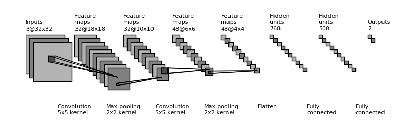
Utilizing the weights sharing strategy, neurons are able to perform convolutions on the data with the convolution filter being formed by the weights. This is then followed by a pooling operation which as a form of non-linear down-sampling, progressively reduces the spatial size of the representation thus reducing the amount of computation and parameters in the network.

Existing between the convolution and the pooling layer is an activation function such as the ReLu layer; a non-saturating activation is applied element-wise, i.e. $f(x) = max(0,x)$ thresholding at zero. After several convolutional and pooling layers, the image size (feature map size) is reduced and more complex features are extracted.

Eventually with a small enough feature map, the contents are squashed into a one dimension vector and fed into a fully-connected MLP for processing. The last layer of this fully-connected MLP seen as the output, is a loss layer which is used to specify how the network training penalizes the deviation between the predicted and true labels.

Before we begin lets take look at the mathematical definitions of convolution and cross-correlation:

Cross-correlation

Given an input image $I$ and a filter (kernel) $K$ of dimensions $k_1 \times k_2$, the cross-correlation operation is given by:

$$\begin{align} (I \otimes K)_{ij} &= \sum_{m = 0}^{k_1 - 1} \sum_{n = 0}^{k_2 - 1} I(i+m, j+n)K(m,n) \tag {1} \end{align}$$

Convolution

Given an input image $I$ and a filter (kernel) $K$ of dimensions $k_1 \times k_2$, the convolution operation is given by:

$$\begin{align} (I \ast K)_{ij} &= \sum_{m = 0}^{k_1 - 1} \sum_{n = 0}^{k_2 - 1} I(i-m, j-n)K(m,n) \tag {2} \\ &= \sum_{m = 0}^{k_1 - 1} \sum_{n = 0}^{k_2 - 1} I(i+m, j+n)K(-m,-n) \tag {3} \end{align}$$

From Eq. $\text{3}$ it is easy to see that convolution is the same as cross-correlation with a flipped kernel i.e: for a kernel $K$ where $K(-m,-n) == K(m,n)$.

Convolution Neural Networks - CNNs

CNNs consists of convolutional layers which are characterized by an input map $I$, a bank of filters $K$ and biases $b$.

In the case of images, we could have as input an image with height $H$, width $W$ and $C = 3$ channels (red, blue and green) such that $I \in \mathbb{R}^{H \times W \times C}$. Subsequently for a bank of $D$ filters we have $K \in \mathbb{R}^{k_1 \times k_2 \times C \times D}$ and biases $b \in \mathbb{R}^{D}$, one for each filter.

The output from this convolution procedure is as follows:

$$\begin{align} (I \ast K)_{ij} &= \sum_{m = 0}^{k_1 - 1} \sum_{n = 0}^{k_2 - 1} \sum_{c = 1}^{C} K_{m,n,c} \cdot I_{i+m, j+n, c} + b \tag {4} \end{align}$$

The convolution operation carried out here is the same as cross-correlation, except that the kernel is “flipped” (horizontally and vertically).

For the purposes of simplicity we shall use the case where the input image is grayscale i.e single channel $C = 1$. The Eq. $\text{4}$ will be transformed to:

$$\begin{align} (I \ast K)_{ij} &= \sum_{m = 0}^{k_1 - 1} \sum_{n = 0}^{k_2 - 1} K_{m,n} \cdot I_{i+m, j+n} + b \tag {5} \end{align}$$

Notation

To help us explore the forward and backpropagation, we shall make use of the following notation:

1. $l$ is the $l^{th}$ layer where $l=1$ is the first layer and $l=L$ is the last layer.
2. Input $x$ is of dimension $H \times W$ and has $i$ by $j$ as the iterators
3. Filter or kernel $w$ is of dimension $k_1 \times k_2$ has $m$ by $n$ as the iterators
4. $w_{m,n}^l$ is the weight matrix connecting neurons of layer $l$ with neurons of layer $l-1$.
5. $b^l$ is the bias unit at layer $l$.
6. $x_{i,j}^l$ is the convolved input vector at layer $l$ plus the bias represented as $$ \begin{align} x_{i,j}^l = \sum_{m}\sum_{n} w_{m,n}^l o_{i + m,j + n}^{l-1} + b^l \end{align} $$
7. $o_{i,j}^l$ is the output vector at layer $l$ given by $$ \begin{align} o_{i,j}^l = f(x_{i,j}^{l}) \end{align} $$
8. $f(\cdot)$ is the activation function. Application of the activation layer to the convolved input vector at layer $l$ is given by $f(x_{i,j}^{l})$

Foward Propagation

To perform a convolution operation, the kernel is flipped $180^\circ$ and slid across the input feature map in equal and finite strides. At each location, the product between each element of the kernel and the input input feature map element it overlaps is computed and the results summed up to obtain the output at that current location.

This procedure is repeated using different kernels to form as many output feature maps as desired. The concept of weight sharing is used as demonstrated in the diagram below:

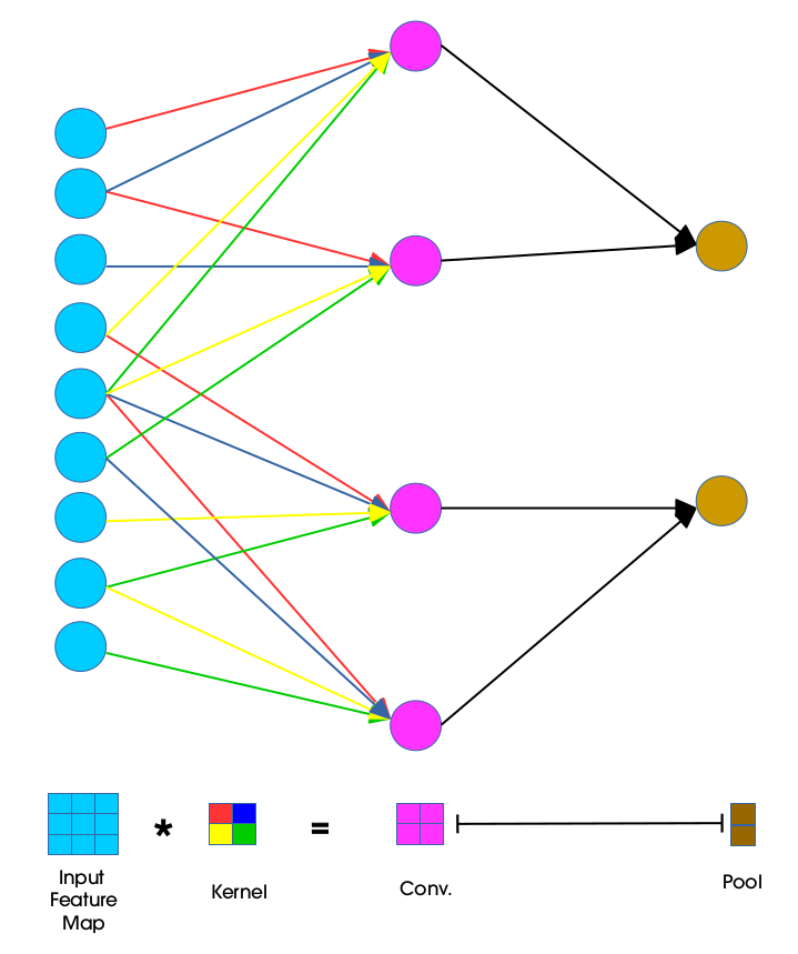
Units in convolutional layer illustrated above have receptive fields of size 4 in the input feature map and are thus only connected to 4 adjacent neurons in the input layer. This is the idea of sparse connectivity in CNNs where there exists local connectivity pattern between neurons in adjacent layers.

The color codes of the weights joining the input layer to the convolutional layer show how the kernel weights are distributed (shared) amongst neurons in the adjacent layers. Weights of the same color are constrained to be identical.

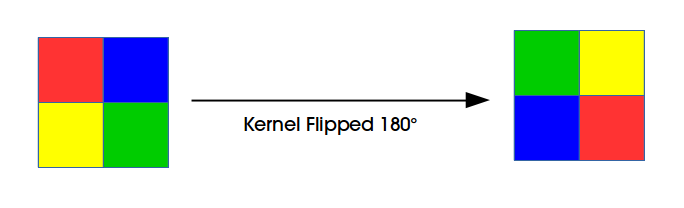
The convolution process here is usually expressed as a cross-correlation but with a flipped kernel. In the diagram below we illustrate a kernel that has been flipped both horizontally and vertically:

The convolution equation of the input at layer $l$ is given by:

$$\begin{align} x_{i,j}^l &= \text{rot}_{180^\circ} \left\{ w_{m,n}^l \right\} \ast o_{i,j}^{l-1} + b_{i,j}^l \tag {6} \\ x_{i,j}^l &= \sum_{m} \sum_{n} w_{m,n}^l o_{i+m,j+n}^{l-1} + b_{i,j}^l \tag {7} \\ o_{i,j}^l &= f(x_{i,j}^l) \tag {8} \end{align}$$

This is illustrated below:

Error

For a total of $P$ predictions, the predicted network outputs $y_p$ and their corresponding targeted values $t_p$ the the mean squared error is given by: $$ \begin{align} E &= \frac{1}{2}\sum_{p} \left(t_p - y_p \right)^2 \tag {9} \end{align} $$

Learning will be achieved by adjusting the weights such that $y_p$ is as close as possible or equals to corresponding $t_p$. In the classical backpropagation algorithm, the weights are changed according to the gradient descent direction of an error surface $E$.

Backpropagation

For backpropagation there are two updates performed, for the weights and the deltas. Lets begin with the weight update.

We are looking to compute $\frac{\partial E}{\partial w_{m^{\prime},n^{\prime}}^l}$ which can be interpreted as the measurement of how the change in a single pixel $w_{m^{\prime},n^{\prime}}$ in the weight kernel affects the loss function $E$.

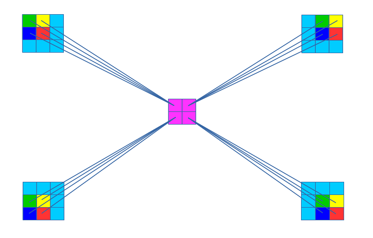
During forward propagation, the convolution operation ensures that the yellow pixel $w_{m^{\prime},n^{\prime}}$ in the weight kernel makes a contribution in all the products (between each element of the weight kernel and the input feature map element it overlaps). This means that pixel $w_{m^{\prime},n^{\prime}}$ will eventually affect all the elements in the output feature map.

Convolution between the input feature map of dimension $H \times W$ and the weight kernel of dimension $k_1 \times k_2$ produces an output feature map of size $\left( H - k_1 + 1 \right)$ by $\left( W - k_2 + 1 \right)$. The gradient component for the individual weights can be obtained by applying the chain rule in the following way:

$$\begin{align} \frac{\partial E}{\partial w_{m^{\prime},n^{\prime}}^l} &= \sum_{i=0}^{H-k_1} \sum_{j=0}^{W-k_2} \frac{\partial E}{\partial x_{i,j}^{l}} \frac{\partial x_{i,j}^{l}}{\partial w_{m^{\prime},n^{\prime}}^l} \\ &= \sum_{i=0}^{H-k_1} \sum_{j=0}^{W-k_2} \delta^{l}_{i,j} \frac{\partial x_{i,j}^{l}}{\partial w_{m^{\prime},n^{\prime}}^l} \tag {10} \end{align}$$

In Eq. $10 \, \text{,} \, x_{i,j}^{l}$ is equivalent to $\sum_{m} \sum_{n} w_{m,n}^{l}o_{i+m,j+n}^{l-1} + b^l$ and expanding this part of the equation gives us:

$$\begin{align} \frac{\partial x_{i,j}^{l}}{\partial w_{m^{\prime},n^{\prime}}^l} = \frac{\partial}{\partial w_{m^{\prime},n^{\prime}}^l}\left( \sum_{m} \sum_{n} w_{m,n}^{l}o_{i+m, j+n}^{l-1} + b^l \right) \tag {11} \end{align}$$

Further expanding the summations in Eq. $11$ and taking the partial derivatives for all the components results in zero values for all except the components where $m = m'$ and $n = n'$ in $w_{m,n}^{l}o_{i+m,j+n}^{l-1}$ as follows:

$$\begin{align} \frac{\partial x_{i,j}^{l}}{\partial w_{m^{\prime},n^{\prime}}^l} &= \frac{\partial}{\partial w_{m',n'}^l}\left( w_{0,0}^{l} o_{ i + 0, j + 0}^{l-1} + \dots + w_{m',n'}^{l} o_{ i + m^{\prime}, j + n^{\prime}}^{l-1} + \dots + b^l\right) \\ &= \frac{\partial}{\partial w_{m^{\prime},n^{\prime}}^l}\left( w_{m^{\prime},n^{\prime}}^{l} o_{ i + m^{\prime}, j + n^{\prime}}^{l-1}\right) \\ &= o_{i+m^{\prime},j+n^{\prime}}^{l-1} \tag {12} \end{align}$$

Substituting Eq. $12$ in Eq. $10$ gives us the following results:

$$\begin{align} \frac{\partial E}{\partial w_{m',n'}^l} &= \sum_{i=0}^{H-k_1} \sum_{j=0}^{W-k_2} \delta^{l}_{i,j} o_{ i + m^{\prime}, j + n^{\prime}}^{l-1} \tag {13} \\ &= \text{rot}_{180^\circ} \left\{ \delta^{l}_{i,j} \right\} \ast o_{m^{\prime},n^{\prime}}^{l-1} \tag {14} \end{align}$$

The dual summation in Eq. $13$ is as a result of weight sharing in the network (same weight kernel is slid over all of the input feature map during convolution). The summations represents a collection of all the gradients $\delta^{l}_{i,j}$ coming from all the outputs in layer $l$.

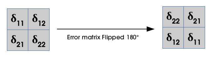
Obtaining gradients w.r.t to the filter maps, we have a cross-correlation which is transformed to a convolution by “flipping” the delta matrix $\delta^{l}_{i,j}$ (horizontally and vertically) the same way we flipped the filters during the forward propagation.

An illustration of the flipped delta matrix is shown below:

The diagram below shows gradients $(\delta_{11}, \delta_{12}, \delta_{21}, \delta_{22})$ generated during backpropagation:

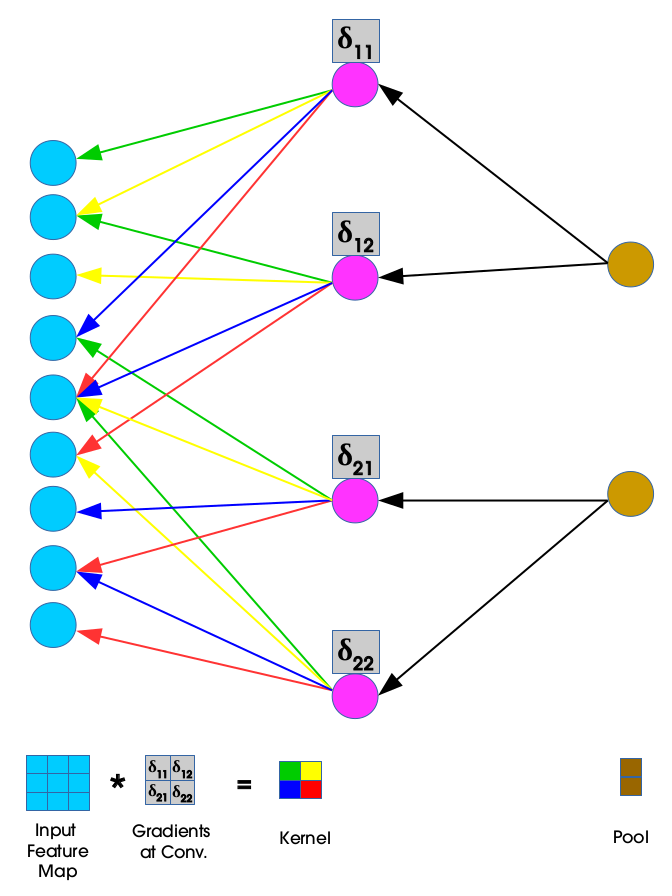
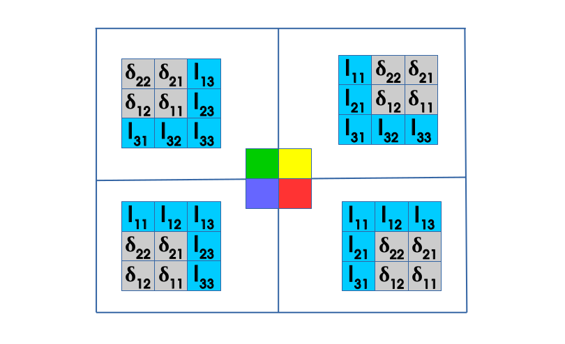
The convolution operation used to obtain the new set of weights as is shown below:

During the reconstruction process, the deltas $(\delta_{11}, \delta_{12}, \delta_{21}, \delta_{22})$ are used. These deltas are provided by an equation of the form:

$\begin{align} \delta^{l}_{i,j} &= \frac{\partial E}{\partial x_{i,j}^{l}} \tag {15} \end{align} \ $

At this point we are looking to compute $\frac{\partial E}{\partial x_{i^{\prime},j^{\prime}}^l}$ which can be interpreted as the measurement of how the change in a single pixel $x_{i^{\prime},j^{\prime}}$ in the input feature map affects the loss function $E$.

From the diagram above, we can see that region in the output affected by pixel $x_{i^{\prime},j^{\prime}}$ from the input is the region in the output bounded by the dashed lines where the top left corner pixel is given by $\left(i^{\prime}-k_1+1,j^{\prime}-k_2+1 \right)$ and the bottom right corner pixel is given by $\left(i^{\prime},j^{\prime} \right)$.

Using chain rule and introducing sums give us the following equation:

$$\begin{align} \frac{\partial E}{\partial x_{i',j'}^{l}} &= \sum_{i,j \in Q} \frac{\partial E}{\partial x_{Q}^{l+1}}\frac{\partial x_{Q}^{l+1}}{\partial x_{i',j'}^l} \\ &= \sum_{i,j \in Q} \delta^{l+1}_{Q} \frac{\partial x_{Q}^{l+1}}{\partial x_{i',j'}^l} \tag{16} \\ \end{align}$$

$Q$ in the summation above represents the output region bounded by dashed lines and is composed of pixels in the output that are affected by the single pixel $x_{i',j'}$ in the input feature map. A more formal way of representing Eq. $16$ is:

$$\begin{align} \frac{\partial E}{\partial x_{i',j'}^{l}} &= \sum_{m = 0}^{k_1 -1} \sum_{n = 0}^{k_2 -1} \frac{\partial E}{\partial x_{i'-m, j'-n}^{l+1}}\frac{\partial x_{i'-m, j'-n}^{l+1}}{\partial x_{i',j'}^l} \\ &= \sum_{m = 0}^{k_1 -1} \sum_{n = 0}^{k_2 -1} \delta^{l+1}_{i'-m, j'-n} \frac{\partial x_{i'-m, j'-n}^{l+1}}{\partial x_{i',j'}^l} \tag{17} \\ \end{align}$$

In the region $Q$, the height ranges from $i' - 0$ to $i' - (k_1 - 1)$ and width $j' - 0$ to $j' - (k_2 - 1)$. These two can simply be represented by $i' - m$ and $j' - n$ in the summation since the iterators $m$ and $n$ exists in the following similar ranges from $0 \leq m \leq k_1 - 1$ and $0 \leq n \leq k_2 - 1$.

In Eq. $17 \, \text{,} \, x_{i^{\prime} - m, j^{\prime} - n}^{l+1}$ is equivalent to $\sum_{m'} \sum_{n'} w_{m^{\prime},n^{\prime}}^{l+1}o_{i^{\prime} - m + m',j^{\prime} - n + n'}^{l} + b^{l+1}$ and expanding this part of the equation gives us:

$$\begin{align} \frac{\partial x_{i'-m,j'-n}^{l+1}}{\partial x_{i',j'}^l} &= \frac{\partial}{\partial x_{i',j'}^l} \left( \sum_{m'} \sum_{n'} w_{m', n'}^{l+1} o_{i' - m + m',j' - n + n'}^{l} + b^{l+1} \right) \\ &= \frac{\partial}{\partial x_{i',j'}^l}\left( \sum_{m'} \sum_{n'} w_{m',n'}^{l+1}f\left(x_{i' - m + m',j' - n + n'}^{l}\right) + b^{l+1} \right) \tag{18} \end{align}$$

Further expanding the summation in Eq. $17$ and taking the partial derivatives for all the components results in zero values for all except the components where $m' = m$ and $n' = n$ so that $f\left(x_{i' - m + m',j' - n + n'}^{l}\right)$ becomes $f\left(x_{i',j'}^{l}\right)$ and $w_{m',n'}^{l+1}$ becomes $w_{m,n}^{l+1}$ in the relevant part of the expanded summation as follows:

$$\begin{align} \frac{\partial x_{i^{\prime} - m,j^{\prime} - n}^{l+1}}{\partial x_{i',j'}^l} &= \frac{\partial}{\partial x_{i',j'}^l}\left( w_{m',n'}^{l+1} f\left(x_{ 0 - m + m', 0 - n + n'}^{l}\right) + \dots + w_{m,n}^{l+1} f\left(x_{i',j'}^{l}\right) + \dots + b^{l+1}\right) \\ &= \frac{\partial}{\partial x_{i',j'}^l}\left( w_{m,n}^{l+1} f\left(x_{i',j'}^{l} \right) \right) \\ &= w_{m,n}^{l+1} \frac{\partial}{\partial x_{i',j'}^l} \left( f\left(x_{i',j'}^{l} \right) \right) \\ &= w_{m,n}^{l+1} f'\left(x_{i',j'}^{l}\right) \tag{19} \end{align}$$

Substituting Eq. $19$ in Eq. $17$ gives us the following results:

$$\begin{align} \frac{\partial E}{\partial x_{i',j'}^{l}} &= \sum_{m = 0}^{k_1 - 1} \sum_{n = 0}^{k_2 - 1} \delta^{l+1}_{i^{\prime} - m,j^{\prime} - n} w_{m,n}^{l+1} f'\left(x_{i',j'}^{l}\right) \tag{20} \\ \end{align}$$

For backpropagation, we make use of the flipped kernel and as a result we will now have a convolution that is expressed as a cross-correlation with a flipped kernel:

$$\begin{align} \frac{\partial E}{\partial x_{i',j'}^{l}} &= \sum_{m = 0}^{k_1 - 1} \sum_{n = 0}^{k_2 - 1} \delta^{l+1}_{i^{\prime} - m,j^{\prime} - n} w_{m,n}^{l+1} f'\left(x_{i',j'}^{l}\right) \\ & = \text{rot}_{180^\circ} \left\{ \sum_{m = 0}^{k_1 - 1} \sum_{n = 0}^{k_2 - 1} \delta^{l+1}_{i^{\prime} + m,j^{\prime} + n} w_{m,n}^{l+1} \right\} f'\left(x_{i',j'}^{l}\right) \tag{21} \\ &= \delta^{l+1}_{i',j'} \ast \text{rot}_{180^\circ} \left\{ w_{m,n}^{l+1} \right\} f'\left(x_{i',j'}^{l} \right) \tag{22} \end{align}$$

Pooling Layer

The function of the pooling layer is to progressively reduce the spatial size of the representation to reduce the amount of parameters and computation in the network, and hence to also control overfitting. No learning takes place on the pooling layers [2].

Pooling units are obtained using functions like max-pooling, average pooling and even L2-norm pooling. At the pooling layer, forward propagation results in an $N \times N$ pooling block being reduced to a single value - value of the “winning unit”. Backpropagation of the pooling layer then computes the error which is acquired by this single value “winning unit”.

To keep track of the “winning unit” its index noted during the forward pass and used for gradient routing during backpropagation. Gradient routing is done in the following ways:

• Max-pooling - the error is just assigned to where it comes from - the “winning unit” because other units in the previous layer’s pooling blocks did not contribute to it hence all the other assigned values of zero
• Average pooling - the error is multiplied by $\frac{1}{N \times N}$ and assigned to the whole pooling block (all units get this same value).

Conclusion

Convolutional neural networks employ a weight sharing strategy that leads to a significant reduction in the number of parameters that have to be learned. The presence of larger receptive field sizes of neurons in successive convolutional layers coupled with the presence of pooling layers also lead to translation invariance. As we have observed the derivations of forward and backward propagations will differ depending on what layer we are propagating through.

References

1. Dumoulin, Vincent, and Francesco Visin. “A guide to convolution arithmetic for deep learning.” stat 1050 (2016): 23. [PDF]
2. LeCun, Y., Boser, B., Denker, J.S., Henderson, D., Howard, R.E., Hubbard, W.,Jackel, L.D.: Backpropagation applied to handwritten zip code recognition. Neural computation 1(4), 541–551 (1989)
3. Wikipedia page on Convolutional neural network
4. Convolutional Neural Networks (LeNet) deeplearning.net
5. Convolutional Neural Networks UFLDL Tutorial