Initialization Of Deep Feedfoward Networks

Jefkine, 1 August 2016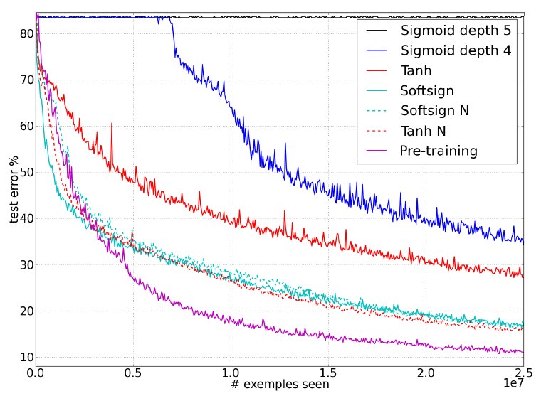

Mathematics Behind Neural Network Weights Initialization - Part Two: In this second of a three part series of posts, we will attempt to go through the weight initialization algorithms as developed by various researchers taking into account influences derived from the evolution of neural network architecture and the activation function in particular.

active region

Introduction

Deep multi-layered neural networks often require experiments that interrogate different initialization routines, activations and variation of gradients across layers during training. These provide valuable insights into what aspects should be improved to aid faster and successful training.

For Xavier and Bengio (2010) [1] the objective was to better understand why standard gradient descent from random initializations was performing poorly in deep neural networks. They carried out analysis driven by investigative experiments that monitored activations (watching for saturations of hidden units) and gradients across layers and across training iterations. They evaluated effects on choices of different activation functions (how it might affect saturation) and initialization procedure (with lessons learned from unsupervised pre-training as a form of initialization that already had drastic impact)

A new initialization scheme that brings substantially faster convergence was proposed. In this article we discuss the algorithm put forward by Xavier and Bengio (2010) [1]

Gradients at Initialization

Earlier on, Bradley (2009) [2] found that in networks with linear activation at each layer, the variance of the back-propagated gradients decreases as we go backwards in the network. Below we will look at theoretical considerations and a derivation of the normalized initialization.

Notation

$f$ is the activation function. For the dense artificial neural network, a symmetric activation function $f$ with unit derivative at $0\,(i.e\, f'(0) = 1)$ is chosen. Hyperbolic tangent and softsign are both forms of symmetric activation functions.
$z^i$ is the activation vector at layer $i$ , $z^i = f(s^{i-1})$
$s^i$ is the argument vector of the activation function at layer $i$ , $s^i = z^{i-1}w^i + b^i$
$w^i$ is the weight vector connecting neurons in layer $i$ with neurons in layer $i+1$ .
$b^i$ is the bias vector on layer $i$ .
$x$ is the network input.

From the notation above, it is easy to derive the following equations of back-propagation

$\begin{align} \frac{\partial Cost}{\partial s_k^{i}} &= f'(s_k^{i}) \sum_{l\in\text{outs}(k)}(w_{k\rightarrow l}^{i+1}) \frac{\partial Cost}{\partial s_k^{i+1}} \tag {1a} \\ \frac{\partial Cost}{\partial s_k^{i}} &= f'(s_k^{i})W_{k,\bullet}^{i+1} \frac{\partial Cost}{\partial s_k^{i+1}} \tag {1b} \\ \frac{\partial Cost}{\partial w_{l,k}^{i}} &= z_l^i\frac{\partial Cost}{\partial s_k^{i}} \tag 2 \end{align}$

The variances will be expressed with respect to the input, output and weight initialization randomness. Considerations made include:

Initialization occurs in a linear regime
Weights are initialized independently
Input feature variances are the same $( =Var[x])$
There is no correlation between our input and our weights and both are zero-mean.
All biases have been initialized to zero.

For the input layer, $X \in \mathbb{R}^{m \times n}$ with $n$ components each from $m$ training samples. Here the neurons are linear with random weights $W^{(in\rightarrow 1)} \in \mathbb{R}^{m \times a}$ outputting $S^{(1)} \in \mathbb{R}^{n \times a}$ .

The output $S^{(1)}$ can be shown by the equations below:

$\begin{align} S^{(1)} &= XW^{(in\rightarrow 1)} \\ S^{(1)}_{ij} =& \sum_{k=1}^m X_{ik}W^{(in\rightarrow 1)}_{kj} \end{align}$

Given $X$ and $W$ are independent, we can show that the variance of their product can be given by:

$\begin{align} \text{Var}(W_iX_i) &= E[X_i]^2 \text{Var}(W_i) + E[W_i]^2 \text{Var}(X_i) + \text{Var}(W_i)\text{Var}(X_i) \tag {3} \end{align}$

Considering our inputs and weights both have mean $0$ , Eqn. $(3)$ simplifies to

$\begin{align} \text{Var}(W_iX_i) &= \text{Var}(W_i)\text{Var}(X_i) \end{align}$

$X_i$ and $W_i$ are all independent and identically distributed, we can therefore show that:

$\begin{align} \text{Var}(\sum_{i=1}^n W_iX_i) &= \text{Var}(W_1X_1 + W_2X_2 + \dotsb + W_n X_n) = n\text{Var}(W_i)\text{Var}(X_i) \end{align} \$

Further, lets now look at two adjacent layers $i$ and $i'$ . Here, $n_i$ is used to denote the size of layer layer $i$ . Applying the derivative of the activation function at $s_k^i$ yields a value of approximately one.

$\begin{align} f'(s_k^{i}) \approx 1, \tag {4} \end{align} \$

Then using our prior knowledge of independent and identically distributed $X_i$ and $W_i$ , we have.

$\begin{align} Var[z^i] &= Var[x] \prod_{i'= 0}^{i-1} n_{i'}Var[W^{i'}] \tag {5} \end{align} \$

$Var[W^{i'}]$ in Eqn. $5$ , is the shared scalar variance of all weights at layer $i'$ . Taking these observations into consideration, a network with $d$ layers, will have the following Eqns.

$\begin{align} Var \left[ \frac{\partial Cost}{\partial s^{i}} \right] &= Var \left[ \frac{\partial Cost}{\partial s^{d}} \right] \prod_{i'= i}^{d} n_{i'+1}Var[W^{i'}], \tag {6} \\ Var \left[ \frac{\partial Cost}{\partial w^{i}} \right] &= \prod_{i'= 0}^{i - 1} n_{i'}Var[W^{i'}] \prod_{i'= i}^{d - 1} n_{i'+1}Var[W^{i'}] \times Var[x] Var \left[ \frac{\partial Cost}{\partial s^{d}} \right]. \tag {7} \end{align}$

We would then like to steady the variance such there is equality from layer to layer. From a foward-propagation point of view, to keep information flowing we would like that

$\begin{align} \forall (i,i'), \, Var[z^i] &= Var[z^{i'}]. \tag {8} \end{align} \$

From a back-propagation point of view, we would like to have:

$\begin{align} \forall (i,i'), \, Var \left[ \frac{\partial Cost}{\partial s^{i}} \right] &= Var \left[ \frac{\partial Cost}{\partial s^{i'}} \right]. \tag {9} \end{align} \$

For Eqns. $(8)$ and $(9)$ to hold, the shared scalar variances $n_{i'}Var[W^{i'}]$ in Eqn. $(5)$ should be $1$ . This is the same as trying to ensure the variances of the input and output are consistent (realize that the technique used here helps avoid reducing or magnifying the signals exponentially hence mitigating the exploding or vanishing gradient problem):

$\begin{align} \forall (i), \quad n_{i}Var[W^{i}] &= 1 \tag {10a} \\ \forall (i), \quad Var[W^{i}] &= \frac{1}{n_{i}} \tag {10b} \\ \forall (i), \quad n_{i+1}Var[W^{i}] &= 1 \tag {11a} \\ \forall (i), \quad Var[W^{i}] &= \frac{1}{n_{i+1}} \tag {11b} \\ \end{align}$

As a compromise between the two constraints (representing back-propagation and foward-propagation), we might want to have $$ \begin{align} \forall (i), \quad \frac{2}{n_{i} + n_{i+1}} \tag {12} \end{align} $$

In the experimental setting chosen by Xavier and Bengio (2010) [1], the standard initialization weights $W_{i,j}$ at each layer using the commonly used heuristic: $$ \begin{align} W_{i,j} \sim U \left[ -\frac{1}{\sqrt n}, \frac{1}{\sqrt n} \right], \tag {13} \end{align} $$

where $U \left[ -\theta, \theta \right]$ is the uniform distribution in the interval $\left(-\theta, \theta \right)$ and $n$ is the size of the previous layer (the number of columns of $W$ ).

For uniformly distributed sets of weights $W \overset{iid}{\sim} U \left[ -\theta, \theta \right]$ with zero mean, we can use the formula $\left\{ x \sim U[a,b] \implies Var[x] = \frac{(b-a)^2}{12} \right\}$ for variance of a uniform distribution to show that:

$\begin{align} Var[W] &= \frac{(2\theta)^2}{12} \\ Var[W] &= \frac{\theta^2}{3} \tag {14} \end{align}$

Substituting Eqn. $(14)$ into an Eqn. of the form $nVar[W] = 1$ yields:

$\begin{align} n\frac{\theta^2}{3} &= 1 \\ \theta^2 &= \frac{3}{n} \\ \theta &= \frac{\sqrt{3}}{\sqrt{n}} \end{align}$

The weights have thus been initialized from the uniform distribution over the interval $$ \begin{align} W \sim U \left[ -\frac{\sqrt 3}{\sqrt {n}}, \frac{\sqrt 3}{\sqrt {n}} \right] \tag{15} \end{align} $$

The normalization factor may therefore be important when initializing deep networks because of the multiplicative effect through layers. The suggestion then is of an initialization procedure that maintains stable variances of activation and back-propagated gradients as one moves up or down the network. This is known as the normalized initialization $$ \begin{align} W \sim U \left[ -\frac{\sqrt 6}{\sqrt {n_{i} + n_{i+1}}}, \frac{\sqrt 6}{\sqrt {n_{i} + n_{i+1}}} \right] \tag{16} \end{align} $$

The normalized initialization is a clear compromise between the two constraints involving $n_{i}$ and $n_{i+1}$ (representing back-propagation and foward-propagation), If you used the input $X \in \mathbb{R}^{m \times n}$ , the normalized initialization would look as follows: $$ \begin{align} W \sim U \left[ -\frac{\sqrt 6}{\sqrt {n + m}}, \frac{\sqrt 6}{\sqrt {n + m}} \right] \tag{17} \end{align} $$

Conclusions

In general, from Xavier and Bengio (2010) [1] experiments we can see that the variance of the gradients of the weights is the same for all the layers, but the variance of the back-propagated gradient might still vanish or explode as we consider deeper networks.

Applications

The initialization routines derived here, more famously known as “Xavier Initialization” have been successfully applied in various deep learning libraries. Below we shall look at Keras a minimalist, highly modular neural networks library, written in Python and capable of running on top of either TensorFlow or Theano.

The initialization routine here is named “glorot_” following the name of one of the authors Xavier Glorot [1]. In the code snippet below, glorot_normal is the implementation of Eqn. $(12)$ while glorot_uniform is the equivalent implementation of Eqn. $(15)$

def get_fans(shape):
    fan_in = shape[0] if len(shape) == 2 else np.prod(shape[1:])
    fan_out = shape[1] if len(shape) == 2 else shape[0]
return fan_in, fan_out

def glorot_normal(shape, name=None):
    ''' Reference: Glorot & Bengio, AISTATS 2010
    '''
    fan_in, fan_out = get_fans(shape)
    s = np.sqrt(2. / (fan_in + fan_out))
    return normal(shape, s, name=name)

def glorot_uniform(shape, name=None):
    fan_in, fan_out = get_fans(shape)
    s = np.sqrt(6. / (fan_in + fan_out))
return uniform(shape, s, name=name)

References

Glorot Xavier, and Yoshua Bengio. “Understanding the difficulty of training deep feedforward neural networks.” Aistats. Vol. 9. 2010. [PDF]
Bradley, D. (2009). Learning in modular systems. Doctoral dissertation, The Robotics Institute, Carnegie Mellon University.
Wikipedia - Variance: “Product of independent variables”.

DeepGrid